11 June 2019
Using Causal Profiling to Optimize the Go HTTP/2 Server
Introduction
If you've been keeping up with this blog, you might be familiar with Causal profiling, a profiling method that aims to bridge the gap between spending cycles on something and that something actually helping improve performance. I've ported this profiling method to Go and figured I'd turn it loose on a real piece of software, The HTTP/2 implementation in the standard library.
HTTP/2
HTTP/2 is a new version of the old HTTP/1 protocol which we know and begrudgingly tolerate. It takes a single connection and multiplexes requests onto it, reducing connection establishing overhead. The Go implementation uses one goroutine per request and a couple more per connection to handle asynchronous communications, having them all coordinate to determine who writes to the connection when.
This structure is a perfect fit for causal profiling. If there is something implicitly blocking progress for a request, it should pop up red hot on the causal profiler, while it might not on the conventional one.
Experiment setup
To grab measurements, I set up an synthetic benchmark with an HTTP/2 server and client. The server takes the headers and body from the Google home page and just writes it for every request it sees. The client asks for the root document, using the client headers from firefox. The client limits itself to 10 requests running concurrently. This number was chosen arbitrarily, but should be enough to keep the CPU saturated.
Causal profiling requires us to instrument the program. We do this by setting Progress markers, which measure the time between 2 points in the code. The HTTP/2 server uses a function called runHandler that runs the HTTP handler in a goroutine. Because we want to measure scheduler latency as well as handler runtime, we set the start of the progress marker before we spawn the goroutine. The end marker is put after the handler has written all its data to the wire.
To get a baseline, let's grab a traditional CPU profile from the server, yielding this profiling graph:
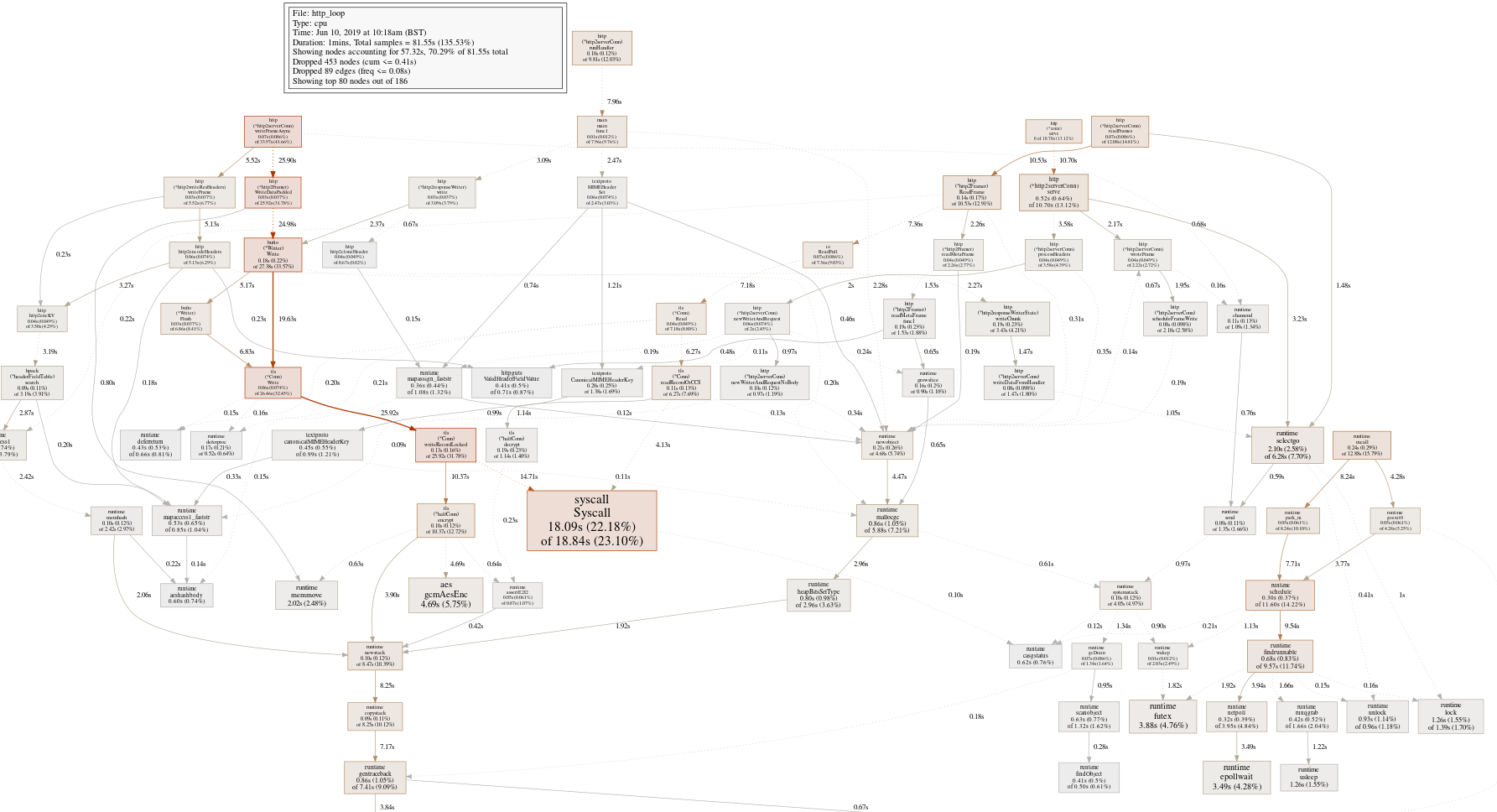
OK, that's mostly what you'd expect from a large well-optimized program, a wide callgraph with not that many obvious places to sink our effort into. The big red box is the syscall leaf, a function we're unlikely to optimize.
The text gives us a few more places to look, but nothing substantial
(pprof) top
Showing nodes accounting for 40.32s, 49.44% of 81.55s total
Dropped 453 nodes (cum <= 0.41s)
Showing top 10 nodes out of 186
      flat  flat%   sum%        cum   cum%
    18.09s 22.18% 22.18%     18.84s 23.10%  syscall.Syscall
     4.69s  5.75% 27.93%      4.69s  5.75%  crypto/aes.gcmAesEnc
     3.88s  4.76% 32.69%      3.88s  4.76%  runtime.futex
     3.49s  4.28% 36.97%      3.49s  4.28%  runtime.epollwait
     2.10s  2.58% 39.55%      6.28s  7.70%  runtime.selectgo
     2.02s  2.48% 42.02%      2.02s  2.48%  runtime.memmove
     1.84s  2.26% 44.28%      2.13s  2.61%  runtime.step
     1.69s  2.07% 46.35%      3.97s  4.87%  runtime.pcvalue
     1.26s  1.55% 47.90%      1.39s  1.70%  runtime.lock
     1.26s  1.55% 49.44%      1.26s  1.55%  runtime.usleep
Mostly runtime and cryptography functions. Let's set aside cryptography, since it will already have been optimized a lot.
Causal Profiling to the rescue
Before we get to the profiling results from causal profiling, it'd be good to have a refresher on how it works. When causal profiling is enabled, a series of experiments are performed. An experiment starts by picking a call-site and some amount of virtual speed-up to apply. Whenever that call-site is executed (which we detect with the profiling infrastructure), we slow down every other executing thread by the virtual speed-up amount.
This would seem counter-intuitive, but since we know how much we slowed down a program when we take our measurement from the Progress marker, we can undo the effect, which gives us the time it would have taken if the chosen call-site was sped up. For a more in-depth look at causal profiling, I suggest you read my other causal profiling posts and the original paper.
The end result is that a causal profile looks like a collection of call-sites, which were sped up by some amount and as a result changed the runtime between Progress markers. For the HTTP/2 server, a call-site might look like:
0x4401ec /home/daniel/go/src/runtime/select.go:73
  0%    2550294ns
 20%    2605900ns    +2.18%    0.122%
 35%    2532253ns    -0.707%    0.368%
 40%    2673712ns    +4.84%    0.419%
 75%    2722614ns    +6.76%    0.886%
 95%    2685311ns    +5.29%    0.74%
For this example, we're looking at an unlock call within the select runtime code. We have the amount that we virtually sped up this call-site, the time it took, the percent difference from the baseline. This call-site doesn't show us much potential for speed-up. It actually shows that if we speed up the select code, we might end up making our program slower.
The fourth column is a bit tricky. It is the percentage of samples that were detected within this call-site, scaled by the virtual speed-up. Roughly, it shows us the amount of speed-up we should expect if we were seeing this as a traditional profile.
Now for a more interesting call-site:
0x4478aa /home/daniel/go/src/runtime/stack.go:881
  0%    2650250ns
  5%    2659303ns    +0.342%    0.84%
 15%    2526251ns    -4.68%    1.97%
 45%    2434132ns    -8.15%    6.65%
 50%    2587378ns    -2.37%    8.12%
 55%    2405998ns    -9.22%    8.31%
 70%    2394923ns    -9.63%    10.1%
 85%    2501800ns    -5.6%    11.7%
This call-site is within the stack growth code and shows that speeding it up might give us some decent results. The fourth column shows that we're essentially running this code as a critical section. With this in mind, let's look back at the traditional profile we collected, now focused on the stack growth code.
(pprof) top -cum newstack
Active filters:
   focus=newstack
Showing nodes accounting for 1.44s, 1.77% of 81.55s total
Dropped 36 nodes (cum <= 0.41s)
Showing top 10 nodes out of 65
      flat  flat%   sum%        cum   cum%
     0.10s  0.12%  0.12%      8.47s 10.39%  runtime.newstack
     0.09s  0.11%  0.23%      8.25s 10.12%  runtime.copystack
     0.80s  0.98%  1.21%      7.17s  8.79%  runtime.gentraceback
         0     0%  1.21%      6.38s  7.82%  net/http.(*http2serverConn).writeFrameAsync
         0     0%  1.21%      4.32s  5.30%  crypto/tls.(*Conn).Write
         0     0%  1.21%      4.32s  5.30%  crypto/tls.(*Conn).writeRecordLocked
         0     0%  1.21%      4.32s  5.30%  crypto/tls.(*halfConn).encrypt
     0.45s  0.55%  1.77%      4.23s  5.19%  runtime.adjustframe
         0     0%  1.77%      3.90s  4.78%  bufio.(*Writer).Write
         0     0%  1.77%      3.90s  4.78%  net/http.(*http2Framer).WriteData
This shows us that newstack is being called from writeFrameAsync. It is called in the goroutine that's spawned every time the HTTP/2 server wants to send a frame to the client. Only one writeFrameAsync can run at any given time and if a handler is trying to send more frames down the wire, it will be blocked until writeFrameAsync returns.
Because writeFrameAsync goes through several logical layers, it uses a lot of stack and stack growth is inevitable.
Speeding up the HTTP/2 server by 28.2% because I felt like it
If stack growth is slowing us down, then we should find some way of avoiding it. writeFrameAsync gets called on a new goroutine every time, so we pay the price of the stack growth on every frame write.
Instead, if we reuse the goroutine, we only pay the price of stack growth once and every subsequent write will reuse the now bigger stack. I made this modification to server and the causal profiling baseline turned from 2.650ms to 1.901ms, a reduction of 28.2%.
A bit caveat here is that HTTP/2 servers usually don't run full speed on localhost. I suspect if this was hooked up to the internet, the gains would be a lot less because the stack growth CPU time would get hidden in the network latency.
Conclusion
It's early days for causal profiling, but I think this small example does show off the potential it holds. If you want to play with causal profiling, you can check out my branch of the Go project with causal profiling added. You can also suggest other benchmarks for me to look at and we can see what comes from it.
P.S. I am currently between jobs and looking for work. If you'd be interested in working with low-level knowledge of Go internals and distributed systems engineering, check out my CV and send me an email on daniel@lasagna.horse.
9 October 2018
The anatomy of a silly hack
Introduction
I recently deployed a small hack on my personal website. In short it enables this:
[daniel@morslaptop ~]$ dig LOC iss.morsmachine.dk

; <<>> DiG 9.11.4-P1-RedHat-9.11.4-2.P1.fc27 <<>> LOC iss.morsmachine.dk
;; global options: +cmd
;; Got answer:
;; ->>HEADER<<- opcode: QUERY, status: NOERROR, id: 62528
;; flags: qr rd ra; QUERY: 1, ANSWER: 1, AUTHORITY: 0, ADDITIONAL: 1

;; OPT PSEUDOSECTION:
; EDNS: version: 0, flags:; udp: 512
;; QUESTION SECTION:
;iss.morsmachine.dk.        IN    LOC

;; ANSWER SECTION:
iss.morsmachine.dk.    4    IN    LOC    43 46 46.715 S 145 49 45.069 W 417946.18m 1m 1m 1m

;; Query time: 42 msec
;; SERVER: 8.8.8.8#53(8.8.8.8)
;; WHEN: Tue Oct 09 12:04:02 BST 2018
;; MSG SIZE  rcvd: 75
I am tracking the location of the International Space station via DNS. This might raise some questions like "Why does DNS have the ability to represent location?", "how the hell are you finding the location of the ISS?" and "Why would you willingly run DNS infrastructure in the Year of Our Lord 2018?".
DNS LOC records
DNS LOC records are mostly a historical oddity that lets you specify a location on earth. Back in the infancy of computer networking, when everybody wasn't sold on the whole TCP/IP thing yet, ferrying email between computers was handled through UUCP. UUCP worked by periodically talking to nearby systems and exchanging any email that needed to be forwarded.
To send an email, you'd have to look up a path from your location to the computer system of the recipient.
You'd then address the email to host!foo!bar!dest_host!recipient. To figure out the path, map files were created that included basic information like the administrative contact, the phone number to call when your email was delayed and in some cases, the location of the server.
Meanwhile, the DNS system was being developed. DNS was meant to replace the HOSTS.TXT file used in TCP/IP networks that mapped user-readable names to IP addresses. To establish feature parity with old UUCP maps, an RFC was written that let you point out where your server is on a map. These LOC records are 16 byte binary representations of latitude, longitude, height above sea level and precision information
I don't know why they included the altitude of the server in the format. I guess people were going to use it to say whether a server was in the basement or on the third floor. For our purposes, the important thing is the range it allows. With a maximum of 42849 kilometers, this easily allows us to represent the location of low-earth orbiting objects.
The international Space Station is one of those objects, so how do we find it?
A brief introduction to the world of orbital mechanics
Tracking satellites in orbit is hard. It usually involves people at NORAD with radars. The good news is that satellites follow the laws of physics and the folks at NORAD are a kindly bunch, who lets us look over their notes.
Every day, they publish new information about the objects in the earths orbit that they track. This data is known as a two-line element set (TLE). The ISS is one of those objects and given a data set, we can predict where the ISS will be sometime in the future.
An aside: TLEs include the year a satellite was launched in its data set and it is specified to have 2 digits. In the leadup to Y2K, there was discussions about changing the TLE format such that it would be able to handle satellites launched after 1999. However, since no artificial satellites existed before 1957, it was decided that any year before 57 would be in the 21st century and any year after would be in the 20th century, solving the problem once and for all!
For the purposes of modeling a satellite orbiting earth, we consider earth as a point mass, with a reference coordinate system where the Z axis points positive through the true north pole and X and Y sits in a plane through the equator. This is known as an earth-centered inertial (ECI) coordinate system and does not rotate with the earth. The model for calculating the future orbit is known as the SGP4/SDP4 algorithms and take into account a whole slew of things, like gravitational effects, atmospheric drag and the shape of the earth. Given the TLE data, we know the orbit and can calculate a future position in the ECI.
The ECI makes orbital calculations easier, because we don't have to handle the rotation of the earth, but we want latitude, longitude and altitude (LLA) for our DNS positioning and latitude is defined by an angular offset to the international meridian. Since we can't stop the world turning, we're forced to do More Maths. Luckily, the angular offset between the reference plane and the meridian can be defined by where the earth is in its rotation around itself and where the earth is in its rotation around the sun. If that all remains the same, then we're all set!
So, we have the position of the ISS, calculated from a TLE in the ECI, converted to LLA and shoved into DNS. Now that we've run out of 3 letter acronyms, let's see how we manage to actually get this thing deployed.
Deploying this thing
Despite my enthusiasm for this project, I do not want to develop a DNS server. The protocol has become a vast, complex mess and I want to offload the effort as much as possible.
PowerDNS provides a good authoritative DNS server that can use remote backends via HTTP. These backends can use a JSON format and I wrote a small HTTP server in Go that responds with custom LOC records that follow the ISS, calculated from a TLE.
Since the SGP4 model is just a model, we have to periodically match it with the physical data to track the ISS accurately. Additionally, the ISS may use its boosters to push it into a higher orbit as it counteracts its orbital decay. Because of this, we fetch new TLEs every day from CelesTrak to make sure that we're following the ISS properly.
The PowerDNS server and my backend HTTP server are deployed as 2 containers in a pod, running on Google Kubernetes Engine. Since my website is managed by Cloudflare, we add an NS record for iss.morsmachine.dk pointing at ns1.morsmachine.dk and an A record for ns1.morsmachine.dk to delegate the responsibility for the subdomain to my new DNS server.
You can try it out by running dig LOC iss.morsmachine.dk in your terminal. You may have to change nameservers if the one on your router doesn't handle DNS esoterica properly.
Sadly, there are a couple of things that I'd like to have added to this hack that weren't possible. GKE doesn't allow you to have a load balanced service that listens on UDP and TCP both on the same IP address which breaks certain DNS operations. Since the LOC record is fairly small, we never actually hit a truncated DNS record and the lack of TCP is mostly a nuisance.
Cloudflare doesn't allow you to specify an A record and NS record for the same domain. Additionally, they don't allow you to proxy wildcard domains unless you are an enterprise customer. Because of this, I couldn't add a small HTTP server to iss.morsmachine.dk that redirected to an explanation and a graphical view like the ISS tracker.
Conclusion
All in all, I'm pretty happy with how this turned out and I learned a bunch about orbital mechanics.
As you've probably guessed by me blogging again: I am looking for work. If you want to work with someone who has knowledge of DNS, Go internals and knows where the HTTP bodies are buried, have a look at my CV and send me an email on daniel@lasagna.horse.
See the index for more articles.